Summer 2016
See the Sweep page for the actual data and plots
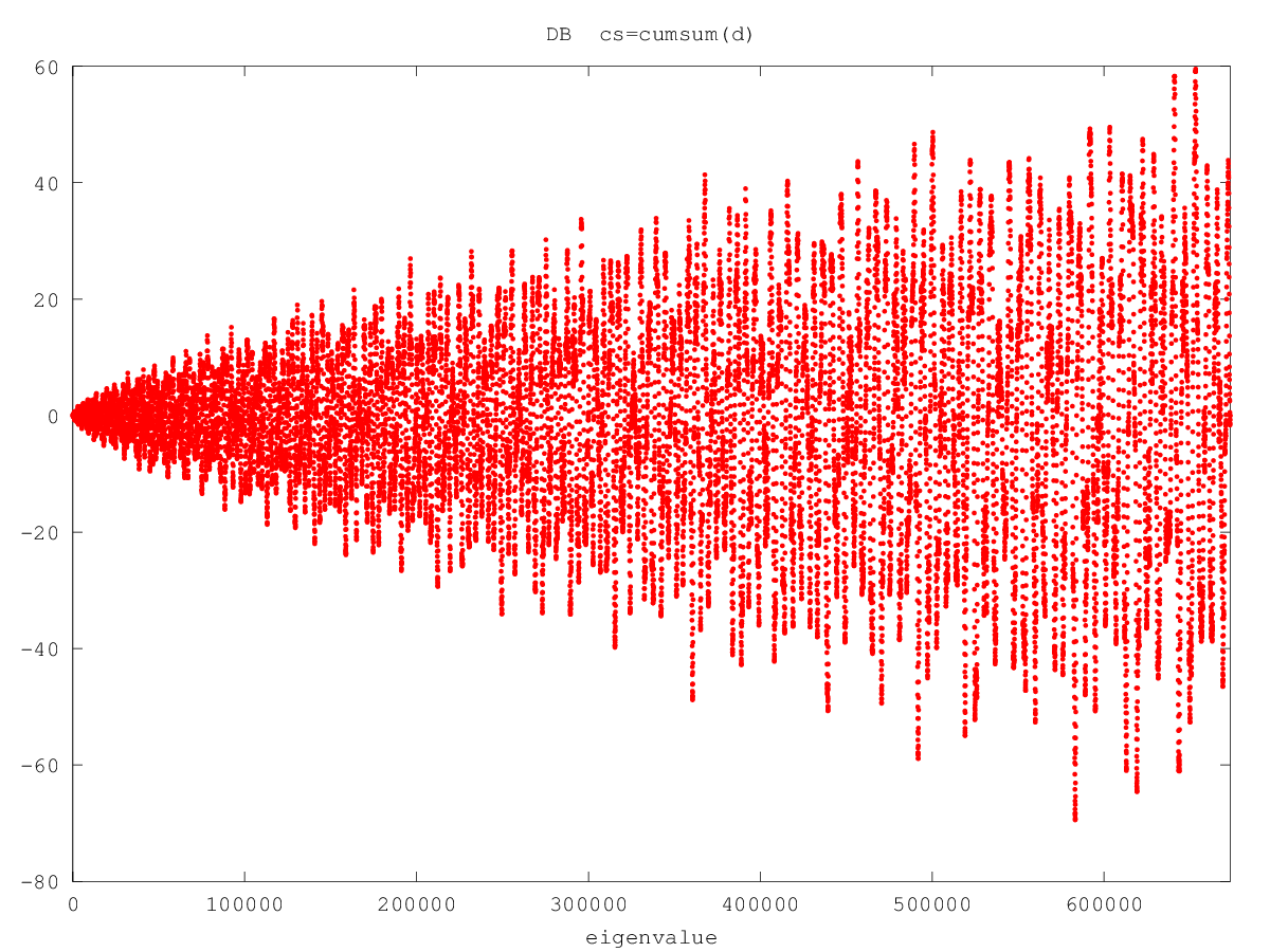
I believe that original material on this page includes the NB, NC, DB, and DC Weyl counting function; and the trivial observation that "cumsum(d)" plot is far more (visually) sensitive to mistakes than the "d" plot, and the related observation that "cumsum(d)" appears to widen linearly.
Weyl counting plot for all of the lowest 164300+ regular pentagon eigenvalues. Includes both Dirichlet and Neumann eigenvalues. These plots have about a quarter of a million data points and are 20000x600 pixels, but file-size is less than 1MB. The very last handful of dots may not be consecutive, and although all eigenvalues are included, some may be misplaced but very slightly.
Weyl's eigenvalue counting formula
Weyl's counting formulas are well known for pure Dirichlet and pure Neumann polygons, but often not (well known) for the polygonal shapes with the relevant boundary/symmetry conditions for the problem at hand.
Of course, Weyl's counting function is approximate and the usual practice is to append an order term, which I will disregard for now. Instead, I will consider only three terms of the form: $$ N_w(\lambda)= c_1\lambda + c_2\sqrt{\lambda}+c_3 $$ where the $c_i$ are three constants. This is called the "two-term" Weyl counting function (because two terms involve $\lambda$), and is the form appropriate to our polygons. This is a smooth function which treats $\lambda\ge 0$ as a continuous eigenparameter. It is supposed to approximate the actual eigenvalue counting function $\#(\lambda)$, which is a step-like function, starting at zero and increasing by $g_i$ (degeneracy of $\lambda_i$) as $\lambda$ increases past the eigenvalue $\lambda_i$.
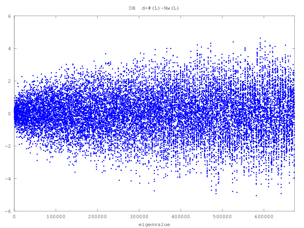
The function $\delta(\lambda)=\#(\lambda)-N_w(\lambda)$ is usually displayed to demonstrate that $N_w(\lambda)$ is correct (for example), and it can be made to have a mean value of zero by appropriately choosing $c_3$.
In our problem, some formulas (specifically, those for DA,NA,DS,NS) can be trivially derived (see Appendix below), but the others (specifically, those for DB,DC,NB,NC) are not obvious to me. Despite that, with a little experience, this is what I came up with: $$ N_w(\lambda) = C+\frac{1}{4\pi}\times \begin{cases} \left[ A \lambda + P \sqrt{\lambda} \right] &\enspace \text{NS} \\ \left[ A \lambda - P \sqrt{\lambda} \right] &\enspace \text{DA} \\ \left[ 2 A \lambda + \sqrt{\lambda} \right] &\enspace \text{NB or NC} \\ \left[ 2 A \lambda - \sqrt{\lambda} \right] &\enspace \text{DB or DC} \\ \left[ A \lambda + (P-1) \sqrt{\lambda} \right] &\enspace \text{DS}\\ \left[ A \lambda - (P-1) \sqrt{\lambda} \right] &\enspace \text{NA} \end{cases} $$ where $P$ is the perimeter and $A$ is the area of the $\pi/2$-$\pi/5$-$3\pi/10$ right triangle with shortest edge equal to 1/2. This triangle is the fundamental domain of the unit-edged regular pentagon according to its dihedral symmetry of order 10. Specifically, those constants are $$ \begin{eqnarray} H &=& \frac{1}{2\tan(\pi/5)} \\ P &=& \frac{1}{2} + H + \sqrt{\frac{1}{4}+H^2} \\ A &=& \frac{1}{8\tan(\pi/5)} \end{eqnarray} $$
Note that the "$(P-1)$" factor scales with the linear dimensions: So if it is doubled so that the new pentagon perimieter doubles and its area becomes four times bigger, then that factor would be "$2(P-1)$" where this $P$ is still the fundamental triangle perimeter of the unit-edged regular pentagon. Similar words apply to the factor of one (before $\sqrt{\lambda}$) in the DB, DC, NB, and NC formulas.
In the Weyl counting function, $C$ is a (possibly) different constant for each of the eight cases. In some cases, it seems easy to calculate exactly, but we don't need to know what it is to make this work.
Adding up all the Dirichlet modes and Neumann modes for the pentagon, respectively, the well-known result is $$ N_w(\lambda) = C + \frac{1}{4\pi}\times \begin{cases} \left[ 10 A \lambda - 5 \sqrt{\lambda} \right] &\enspace \text{Dirichlet }\unicode{x2b20} \\ \left[ 10 A \lambda +5 \sqrt{\lambda} \right] &\enspace \text{Neumann }\unicode{x2b20} \end{cases} $$ where one must not forget to double up the B and C modes since they are doubly degenerate in the pentagon. Note $10A$ is the area and 5 is the the perimeter of the unit-edged regular pentagon, as they should be.
The B and C modes have a sort of periodic-type symmetry condition on some of their symmetry lines, and I don't know how to figure out the Weyl counting function from first principles. However, I'm sure it is possible since I apparently found the answer. Perhaps a starting point is to assume the B and C counting functions are equal to each other (to within an additive constant) for a given pentagon boundary condition, then it is easy to solve.
The Algorithm
To describe in more detail the plots, I use the octave language, which is similar to matlab, but octave is free software (GNU octave). I first give the strategy, then an octave script file, with its graphic output.
First note that there are no accidental degeneracies within the eight towers: The smallest eigenvalue gap happens to be $\delta\lambda\approx 0.164$ (at DB $\lambda\approx 907100$). So, I don't have to deal with such degeneracies right now, but the B and C eigenvalues are actually doubly degenerate in the pentagon.
Put all the eigenvalues of a given tower in an array L. These are indexed beginning from 1 so that 0<L(1)<L(2)<...<L(end).
Define next an index array $\fbox{I=1:length(L);}$, which is simply the vector of numbers [1,2,3,4,...,length(L)]. Notice that I(end)=length(L).
Define the actual counting function $\#(\lambda)$, which is the number of eigenvalues less than (or equal to) $\lambda$. Here $\lambda$ is a continuous parameter starting at zero. For L(n)<$\lambda$<L(n+1), this counting function is equal to n for valid values of n=1,2,3,...,I(end)-1.
What happens exactly at an eigenvalue for $\#(\lambda)$ is not important for this procedure. What we really want to do is adjust our constant $C$ so that the Weyl counting function effectively passes through (on average) the middle of the risers of the steps in $\#(\lambda)$. Below, I impose this convention by subtracting the mean of d0 so that the mean of d is zero.
Now, observe that I(n)=n is also the value of $\#(\lambda)$ for L(n)<$\lambda$<L(n+1). This vector I behaves very much like the actual counting function $\#(\lambda)$, although we have to watch out for n=0 or for n>length(L).
Let Nw0(L) be the Weyl counting vector (where L is our octave vector of eigenvalues), where the constant $C$ is set equal to zero. Then, I can form the difference vector, $\fbox{d0 = I - Nw0(L);}$ where, for clarity, d0(1)=1-Nw0(L(1)), d0(2)=2-Nw0(L(2)), and so on.
If there are no missing eigenvalues (below some specified number), and the Weyl counting function (with $C=0$) is correct, then this vector d0 will appear to fluctuate around a constant (the mean of d0). With this in mind, subtract this constant off so that $\fbox{d = d0 - mean(d0);}$ This vector d has mean of zero.
Finally, when d is plotted versus L, we obtain our "Weyl Plots". If everything worked, they should fluctuate around zero, and not vary very much, even for tens of thousands of eigenvalues. One interesting feature of these plots is that, even though the Weyl counting formula is supposed to be an asymptotic formula (for large $\lambda$), it seems to offer a nice relationship all the way down to $\lambda=0$.
Assume the DB eigenvalues are listed in the file L.DB.dat, which start out like
Because of the script's simplicity, the data file must not have any extra blank lines or extraneous characters.
The octave script might look like the following (for the DB eigenvalues):
|
|
Plotting the cummulative sum of d (cumsum(d)) is also very useful, as illustrated below.
The resulting graphics files are:
| 
|
| plot(L,d,".b"); | plot(L,cumsum(d),".r"); |
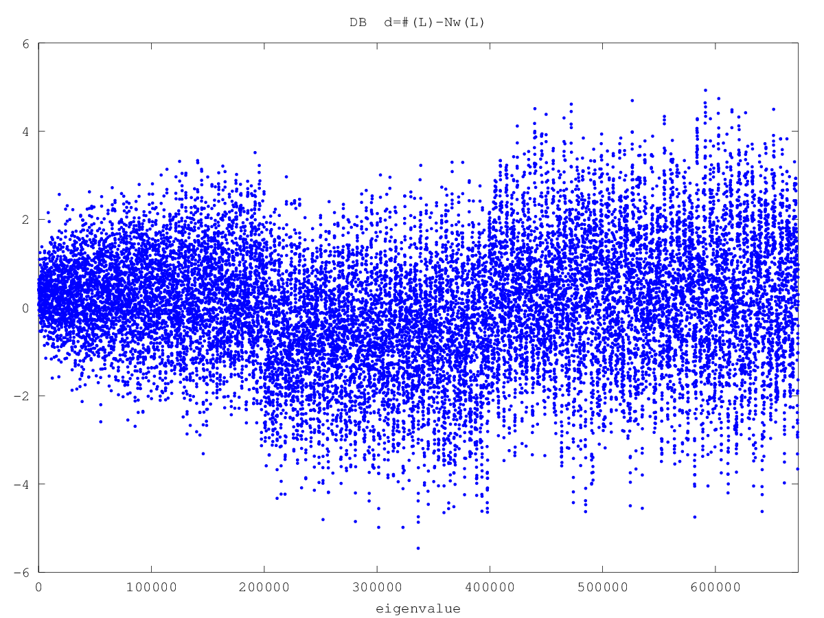
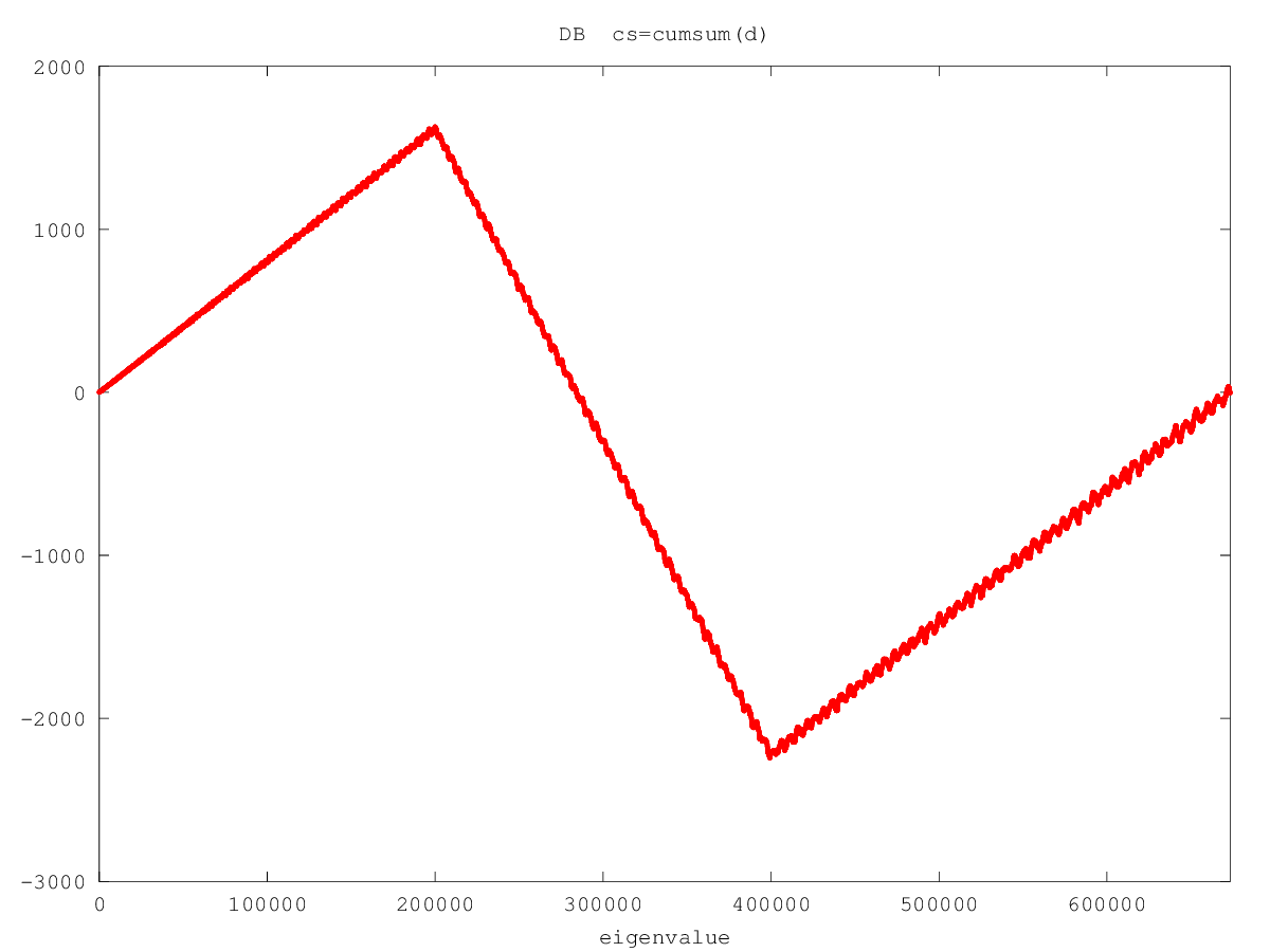
These plots, at first, appear to be simply "noise", which might not seem useful. However, these plots can be very useful to spot mistakes in our data. To demonstrate, I deliberately edit the eigenvalue file to
- remove one eigenvalue, which is 199,963.842, and
- insert one extra (fake) eigenvalue at 400,000.
| 
|
| plot(L,d,".b"); | plot(L,cumsum(d),".r"); |
Those two errors show up in both plots, but far more dramatically in the cumsum plot. By examining the knees in the cumsum plot, it is easy to see where to look for mistakes in the sweep process, here at 200,000 and 400,000. In this example, only two mistakes were deliberately induced, but there are 18,373 eigenvalues in that file: It is extremely senstive to even one or two mistakes. (Using my sweep method, I would typically make about two or three errors like this in each sweep interval of $\delta\lambda=100,000$.)
For these reasons, when doing an eigenvalue calculation like this, it is rather important to make these plots. They don't prove we are right, but they can easily prove we are wrong ... and show us were to find the mistakes.
Another observation worth pursuing is the relatively simple linear widening of the cumsum (for valid data). This is to compare with the much more well known d function, which grows wider, but in a more complicated fashion.
As one final note, if the lowest $N$ eigenvalues are omitted, this process won't detect those omissions (it is absorbed in $C$), but can be used to see that the list that is used is complete. Thus, to be complete, this means we must make sure the lowest eigenvalue is included.
Appendix - Elementary derivation of DA,DS,NA,NS Weyl counting functions
Note: If you understand this without drawing triangles and pentagons, good for you. I need to include some pictures.For a pure Dirichlet or pure Neumann polygon, we have, to within an additive constant, $$ 4\pi N_w(\lambda) = \text{(area)}\lambda \mp \text{(perimeter)}\sqrt{\lambda} $$ where "$-$" is for Dirichlet and "$+$" is for Neumann.
For this section, I adopt the notation that the ordered triple (abc) will represent the even or odd nature of the edges of the $\pi/5$-$\pi/2$-$3\pi/10$ fundamental triangle. They are arranged in order from shortest to longest edges.
I use "e" for even (Neumann) and "o" for odd (Dirichlet). For example, the DS pentagon mode will have (oee), specifically, the shortest edge is odd (Dirichlet boundary condition of the pentagon) and the other two longer edges are even (even symmetry lines of the apothem and radius of pentagon).
The area of this triangle is $A$ and the edges are $\{1/2,H,S\}$ where $S=\sqrt{1/4+H^2}$ and $H$ is given in the octave script above. The perimeter of that fundamental region triangle is $P=1/2+H+S$.
With this notation, and using the fundamental region of that unit-edged regular pentagon, $$ \begin{eqnarray} && \text{NS}\unicode{x2b20}:\enspace 4\pi N_w^\text{(eee)}(\lambda) = A\lambda + (1/2+H+S)\sqrt{\lambda}\\ && \text{DA}\unicode{x2b20}:\enspace 4\pi N_w^\text{(ooo)}(\lambda) = A\lambda - (1/2+H+S)\sqrt{\lambda} \end{eqnarray} $$
To get the DS and NS counting functions, imagine two fundamental region triangles joined together on their shortest edges forming a $\pi/5$-$\pi/5$-$3\pi/5$ isoceles triangle T. The eigenmodes of T are either even or odd due to its simple reflection symmetry. The Dirichlet T modes are the (ooo)+(eoo) modes, and the Neumann T modes are the (oee)+(eee) modes. The (e**) modes are the even T modes and the (o**) are its odd modes.We know the T counting functions since T is a polygon (triangle) with area $2A$, and perimeter $(2H+2S)$. Therefore, $$ \begin{eqnarray} & \text{Neumann T}:\enspace & 4\pi \left( N_w^\text{(oee)}(\lambda)+N_w^\text{(eee)}(\lambda)\right) = (2A)\lambda + (2H+2S)\sqrt{\lambda} \\ & \text{Dirichlet T}:\enspace & 4\pi \left(N_w^\text{(ooo)}(\lambda)+N_w^\text{(eoo)}(\lambda)\right) = (2A)\lambda - (2H+2S)\sqrt{\lambda} \end{eqnarray} $$
When one realizes that the DS$\unicode{x2b20}$ modes are the (oee) modes, and the NA$\unicode{x2b20}$ modes are the (eoo) modes, the above four equations can be used to get $$ \begin{eqnarray} && \text{NA}\unicode{x2b20}:\enspace 4\pi N_w^\text{(eoo)}(\lambda) = A\lambda + ([1/2+H+S]-1)\sqrt{\lambda}\\ && \text{DS}\unicode{x2b20}:\enspace 4\pi N_w^\text{(oee)}(\lambda) = A\lambda - ([1/2+H+S]-1)\sqrt{\lambda} \end{eqnarray} $$ Using $P=1/2+H+S$, we get the four equations for DA,DS,NA,NS given at the beginning of this page.
Mon May 30 16:09:55 UTC 2016
rsjones7 at yahoo dot com